Predicting Stock Prices with Kalman Filters

Introduction

In the dynamic and often unpredictable world of financial markets, accurate stock price prediction remains a holy grail for investors and traders. The challenge lies in the inherent volatility and the multitude of factors influencing stock prices, from company performance and market sentiment to global economic conditions and geopolitical events.

Traditional methods of stock price prediction, such as fundamental analysis and technical analysis, have long been used by investors. However, these approaches often struggle to capture the complex, non-linear dynamics of financial markets. Fundamental analysis, while valuable for long-term investing, can miss short-term price movements. Technical analysis, on the other hand, relies on historical patterns that may not always repeat in the future.

Enter Kalman filters, developed by Rudolf E. Kálmán in 1960. These recursive algorithms are designed to estimate the state of a dynamic system from noisy measurements. Their ability to handle noisy data and adapt to changing systems makes them particularly suitable for stock price prediction, potentially offering a more sophisticated approach to capturing market dynamics.

Originally developed for aerospace applications, Kalman filters have found their way into various fields, including finance. Their strength lies in their ability to combine predictions from a model with new observations, continually updating and improving estimates. This adaptive nature is particularly valuable in the ever-changing landscape of stock markets.

This article will explore how Kalman filters can be applied to stock price prediction, potentially offering traders a more nuanced tool for market analysis and decision-making. We'll delve into the mathematical foundations, implementation details, and practical considerations of using Kalman filters in this context.

From Markov Models to Kalman Filters

To understand Kalman filters, it's helpful to start with simpler concepts and build up to the full model. Let's begin with Markov processes and Hidden Markov Models before introducing Kalman filters.

Markov Process

A Markov process is a sequence of states where each state depends only on the previous state:

\[P(z_t | z_{1:t-1}) = P(z_t | z_{t-1})\]

This property, known as the Markov property, essentially states that the future is independent of the past given the present. In the context of stock prices, this would suggest that tomorrow's price depends only on today's price, not on the entire price history. While this is a simplification, it serves as a useful starting point for modeling.

Hidden Markov Model

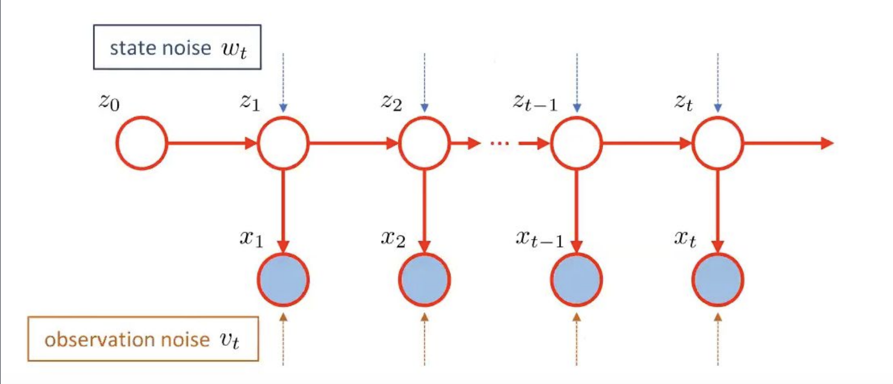
Hidden Markov Models (HMMs) introduce the concept of hidden states and observations:

\[z_t = f(z_{t-1}) + w_t\] \[x_t = h(z_t) + v_t\]

Where \(z_t\) is the hidden state, \(x_t\) is the observation, \(w_t\) is the process noise, and \(v_t\) is the observation noise.

In the context of stock prices, we might think of the hidden state as the "true" value of a stock, which we can't observe directly. What we can observe (the stock price) is a noisy representation of this true value. The process noise represents unpredictable changes in the true value, while the observation noise represents factors that cause the observed price to deviate from the true value.

Kalman Filter

The Kalman filter extends this concept with linear state-space models:

\[z_t = Az_{t-1} + w_t, \quad w_t \sim N(0, Q)\] \[x_t = Hz_t + v_t, \quad v_t \sim N(0, R)\]

Where \(A\) is the state transition matrix, \(H\) is the observation matrix, \(Q\) is the process noise covariance, and \(R\) is the observation noise covariance.

In this model, the state transition (\(A\)) and observation (\(H\)) processes are assumed to be linear, and the noise terms are assumed to be Gaussian. While these assumptions might seem restrictive, they allow for efficient computation and often work well in practice. For stock prices, these linear models can capture trends and mean-reverting behavior.

The Kalman filter operates in two steps:

Prediction Step:

\[\hat{z}_{t|t-1} = A\hat{z}_{t-1|t-1}\] \[P_{t|t-1} = AP_{t-1|t-1}A^T + Q\]

This step predicts the current state based on the previous state. \(\hat{z}_{t|t-1}\) is our prediction of the current state, and \(P_{t|t-1}\) is our estimate of the error in this prediction. The prediction step essentially moves our estimate forward in time, accounting for how we expect the state to change.

Update Step:

\[K_t = P_{t|t-1}H^T(HP_{t|t-1}H^T + R)^{-1}\] \[\hat{z}_{t|t} = \hat{z}_{t|t-1} + K_t(x_t - H\hat{z}_{t|t-1})\] \[P_{t|t} = (I - K_tH)P_{t|t-1}\]

The update step refines our prediction using the actual measurement. \(K_t\) is the Kalman gain, which determines how much we trust the measurement versus our prediction. If our prediction is very uncertain (high \(P_{t|t-1}\)) or our measurement is very precise (low \(R\)), we'll weight the measurement more heavily. Conversely, if our prediction is confident or our measurement is noisy, we'll rely more on the prediction.

This process allows the Kalman filter to continually refine its estimates, balancing between the model's predictions and new observations. In the context of stock prices, this means the filter can adapt to new market information while maintaining a sense of the overall trend. It can potentially capture both the short-term fluctuations and the longer-term trajectory of a stock's price.

Problem Definition

Our goal is to predict future stock prices using Kalman filters. To do this effectively, we need to address some of the challenges inherent in stock price data. One key issue is that stock prices often exhibit increasing variance over time – a phenomenon known as heteroskedasticity. To mitigate this, we use log-transformed prices:

\[y_t = \log(p_t)\]

Where \(p_t\) is the stock price at time \(t\) and \(y_t\) is the log-transformed price.

This transformation has several advantages. It stabilizes the variance, making the data more suitable for our linear Kalman filter model. Additionally, it allows us to model relative changes rather than absolute changes, which often makes more sense for financial data. Furthermore, it ensures that our model will never predict negative prices, which would be nonsensical. These properties make the log transformation particularly useful in financial modeling contexts.

However, it's important to note that this transformation also has some limitations. For instance, it can sometimes underestimate large price movements. Therefore, when interpreting the results, we need to keep in mind that we're working with log prices rather than raw prices.

Implementation

Implementing a Kalman filter for stock price prediction involves several steps. Let's go through each in detail:

Log-Transform Prices

First, we transform our raw price data:

\[y_t = \log(p_t)\]

This is a simple operation, but it's crucial for the reasons discussed earlier.

Initialize Kalman Filter

Next, we need to set up the initial parameters for our Kalman filter:

These choices deserve some explanation:

Optimize Parameters Using the EM Algorithm

While we've made some initial choices for our parameters, we can potentially improve our model by optimizing these parameters based on our data. The Expectation-Maximization (EM) algorithm is a powerful tool for this purpose.

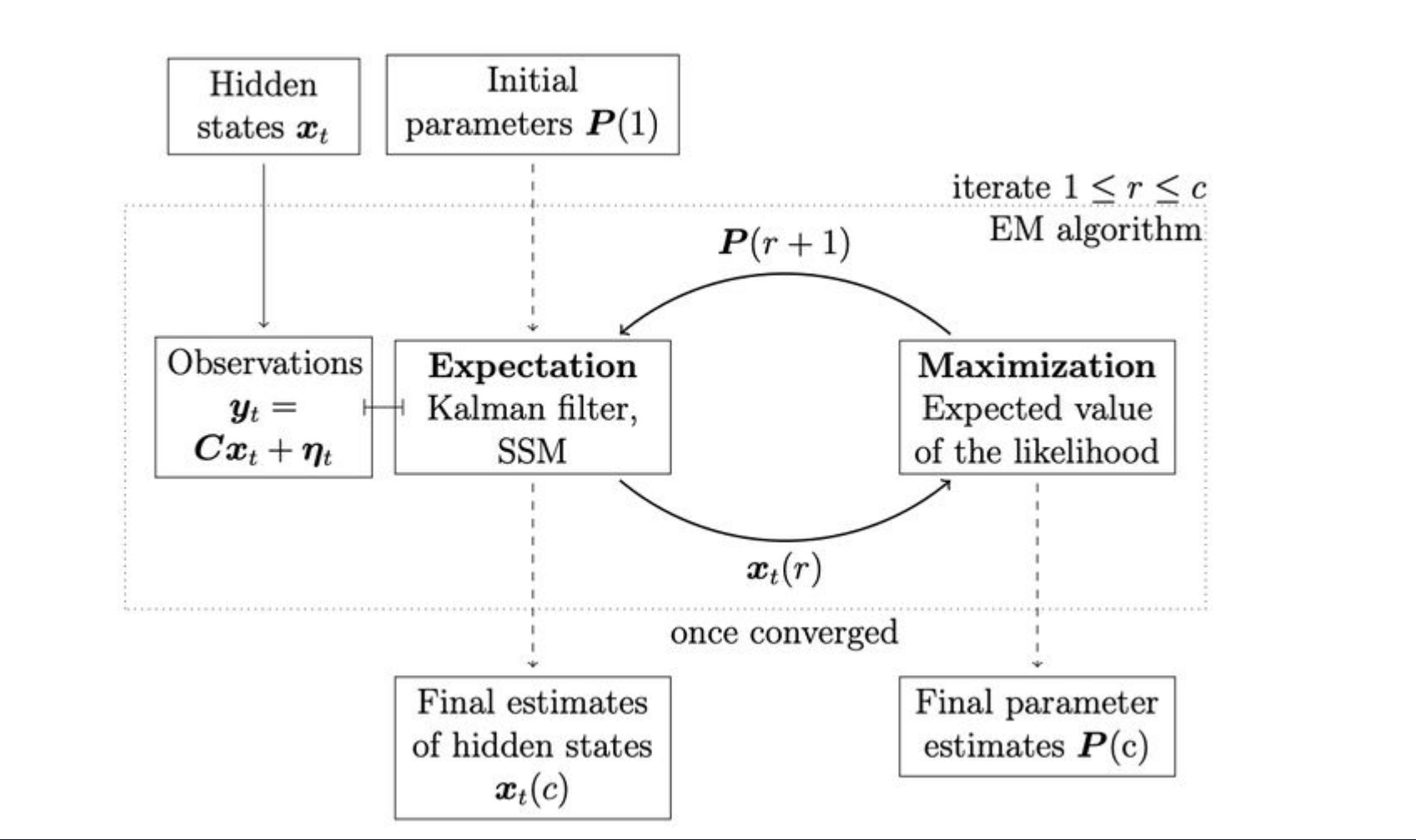
The EM algorithm works by iteratively improving our parameter estimates:

Through this process, we can optimize:

The EM algorithm can help our model better fit the specific characteristics of our stock price data. However, it's important to be cautious of overfitting, especially with limited data.

Predict Future Prices

After optimizing the parameters, we use the Kalman filter to estimate the hidden state for each time step:

\[\hat{y}_t = H\hat{z}_t\]

Then, we convert the log prices back to actual prices:

\[\hat{p}_t = \exp(\hat{y}_t)\]

This gives us our final price predictions.

Python Implementation

import numpy as np
import pandas as pd
from pykalman import KalmanFilter

stock_data = pd.read_csv('VZ_Year.csv')
prices = stock_data['Close'].values
log_prices = np.log(prices)

kf = KalmanFilter(transition_matrices=[1],
                  observation_matrices=[1],
                  initial_state_mean=0,
                  initial_state_covariance=1,
                  observation_covariance=1,
                  transition_covariance=0.0001)

kf = kf.em(log_prices, n_iter=10)

state_means = np.zeros_like(log_prices)
state_covs = np.zeros_like(log_prices)
state_mean = log_prices[0]
state_cov = kf.initial_state_covariance

state_means[0] = state_mean
state_covs[0] = state_cov
mse_list = []

for t in range(i, len(log_prices)):
    state_mean, state_cov = kf.filter_update(state_mean, state_cov, log_prices[t])
    state_means[t] = state_mean
    state_covs[t] = state_cov

    squared_error = (prices[t] - np.exp(state_mean)) ** 2
    mse_list.append(squared_error)
    print(f"Iteration {t}: Squared Error = {float(squared_error):.4f}")

mse = np.mean(mse_list)
print(f"Mean Square Error: {mse:.4f}")

This implementation uses the pykalman library, which provides a convenient interface for working with Kalman filters. The code loads the data, initializes the Kalman filter, optimizes the parameters using EM, and then applies the filter to our data.

Results

After running our Kalman filter on the stock price data, we can visualize the results:

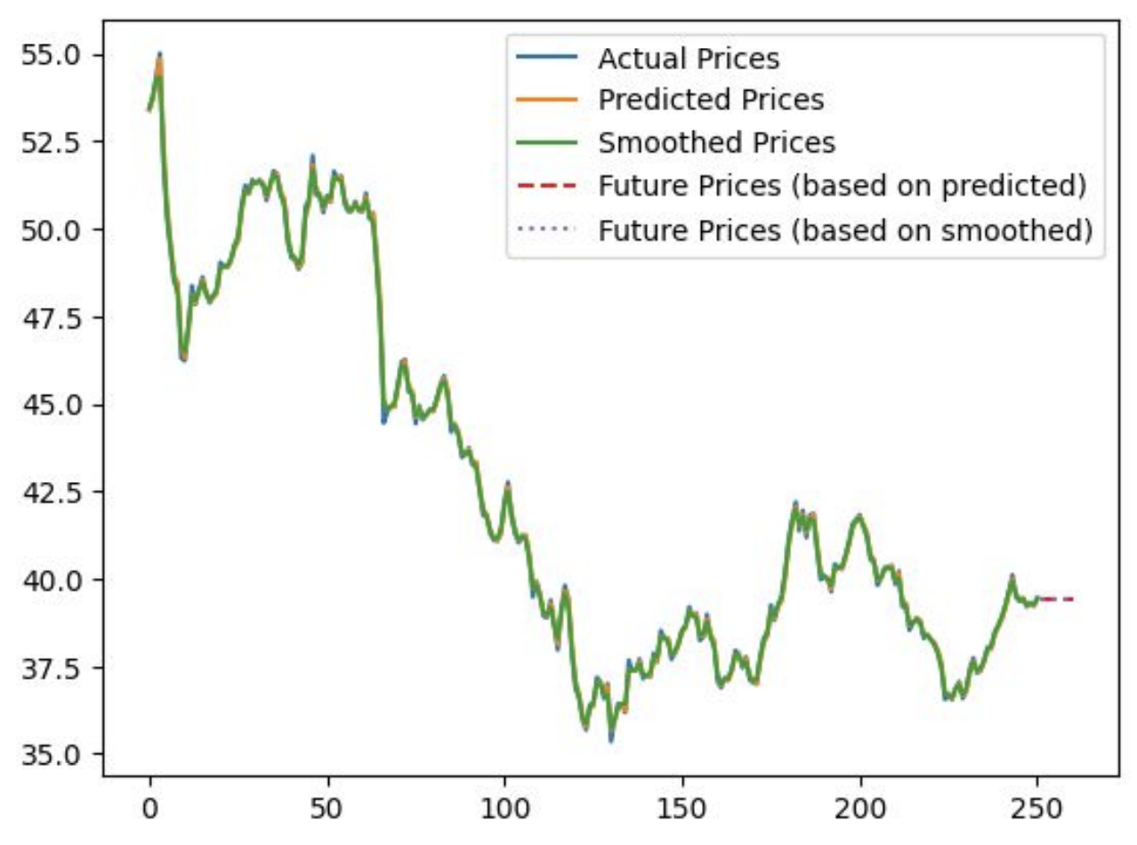
This graph shows the original stock prices compared to the Kalman filter predictions over time. We can see that the Kalman filter provides a smoothed estimate of the stock price, potentially revealing underlying trends that are obscured by day-to-day fluctuations.

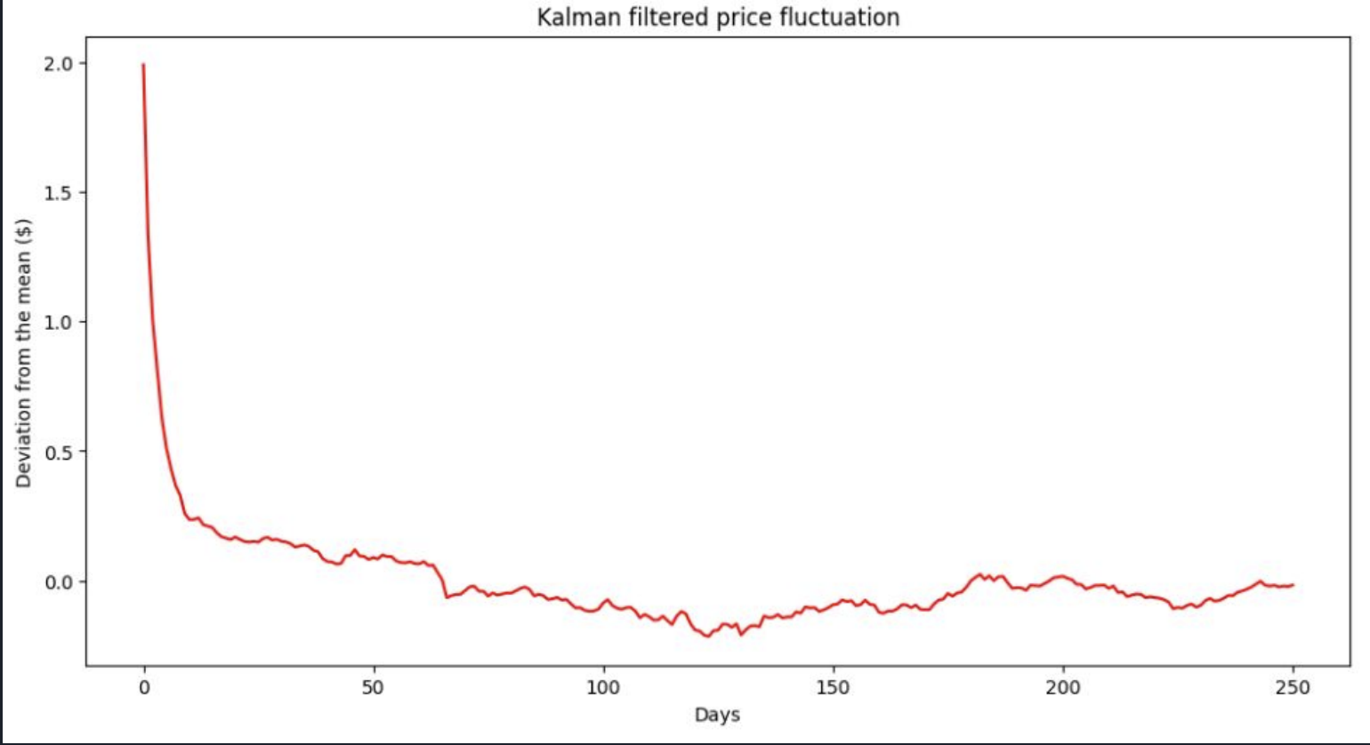
This second graph illustrates how the Kalman filter smooths out price fluctuations. By reducing the impact of short-term noise, the Kalman filter may help identify more persistent price trends.

The last 10 iterations of the EM algorithm showed the following Squared Errors:

Iteration 241: Squared Error = 0.00031
Iteration 242: Squared Error = 0.00074
Iteration 243: Squared Error = 0.00000
Iteration 244: Squared Error = 0.00088
Iteration 245: Squared Error = 0.00028
Iteration 246: Squared Error = 0.00001
Iteration 247: Squared Error = 0.00021
Iteration 248: Squared Error = 0.00002
Iteration 249: Squared Error = 0.00003
Iteration 250: Squared Error = 0.00019
Mean Square Error: 0.0161

The Mean Squared Error (MSE) is calculated as:

\[MSE = \frac{1}{n} \sum_{t=1}^n (y_t - \hat{y}_t)^2\]

Where \(y_t\) is the actual log price and \(\hat{y}_t\) is the estimated log price.

An MSE of 0.0161 suggests that our model's predictions are, on average, quite close to the actual prices. However, it's important to interpret this in context. For stock price prediction, even small errors can be significant, especially when dealing with large trading volumes.

Conclusion

The use of Kalman filters for stock price prediction shows promise. By modeling the hidden state of stock prices and adapting to new observations, Kalman filters can potentially provide more accurate predictions than traditional methods. The ability to smooth out short-term fluctuations while still adapting to changing trends could be particularly valuable for investors looking to understand the underlying dynamics of a stock's price movement.

However, it's crucial to approach these results with caution. Stock prices are influenced by many complex factors, including company performance, market sentiment, economic conditions, and unexpected events. No prediction method, including Kalman filters, can capture all of these factors perfectly.

There are also practical considerations to keep in mind when applying Kalman filters to stock prediction. Computational intensity is one such factor; while not as demanding as some machine learning approaches, Kalman filters still require more computation than simpler forecasting methods. This could be a consideration for high-frequency trading applications. Another important aspect is model updates. The stock market is non-stationary, meaning its statistical properties change over time. Regular re-estimation of the model parameters may be necessary to maintain predictive power. Overfitting is another concern; with any statistical model, there's a risk of overfitting to historical data. Cross-validation and out-of-sample testing are crucial to ensure the model generalizes well. Lastly, Kalman filters, like many statistical models, may struggle to predict or quickly adapt to rare, high-impact events (often called "black swans" in finance).

The Kalman filter approach should be used in conjunction with other analysis techniques and fundamental research for comprehensive investment decision-making. It's a tool that can provide valuable insights, but it shouldn't be relied upon in isolation.

Future research in this area could explore several promising directions. One avenue is incorporating additional features; including other relevant financial indicators or market sentiment data could potentially improve the model's predictive power. Non-linear extensions present another opportunity; techniques like the Extended Kalman Filter or Unscented Kalman Filter could capture non-linear dynamics in stock prices. Exploring multi-dimensional models is also worth considering; applying Kalman filters to multiple related stocks or market indices simultaneously could provide a more comprehensive view of market dynamics. Finally, a rigorous comparison of Kalman filter predictions with other forecasting techniques (e.g., ARIMA models, neural networks) could help understand the relative strengths and weaknesses of each approach.

As we continue to face increasingly complex challenges in financial prediction, techniques like Kalman filters may play a crucial role in developing more sophisticated and accurate trading strategies. By providing a way to balance between model predictions and new observations, Kalman filters offer a flexible and adaptive approach to understanding stock price movements. While they're not a magic solution to the challenges of stock prediction, they represent a valuable addition to the toolbox of quantitative finance.